Radio Effects of the Total Eclipse of 1999 and How to Observe them

G, H. Grayer BSc PhD, G3NAQ

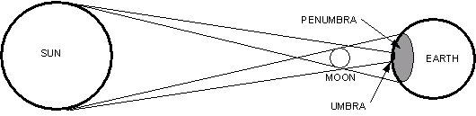
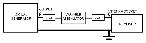
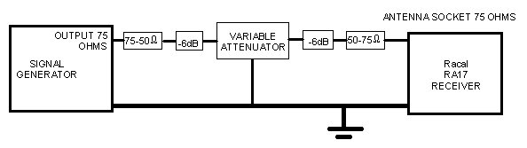
WARNING! THIS ARTICLE DEALS ONLY WITH OBSERVING THE ECLIPSE BY RADIO WAVES. IF HOWEVER YOU INTEND TO OBSERVE THE ECLIPSE VISUALLY, ACT BY THE OFFICIAL ADVICE GIVEN IN E.G. REFERENCES [1,7]. OTHERWISE YOUR SIGHT COULD BE AT RISK. Part 1. THE ECLIPSE AND ITS EFFECTS Introduction For most people the eclipse of 1999 August will be a once-in-a-lifetime occasion, for this will be the first time for 72 years that a total eclipse has been visible from mainland UK, and the next one will not occur until 2090. Fig. 1 shows superimposed on the map of Europe the path of totality [1] - where the sun is complete covered at some instant - while the rest is in the region of partiality , where the sun will be seen to be only partly obscured. This partial shadow is known as the penumbra , while the complete shadow is called the umbra. Why is a solar eclipse so rare? The moon orbits the earth in just over 27 days, so that once every lunar month it is in the general direction of the sun. However, the lunar orbit is not in the same plane as that of the sun, so usually the moon passes above or below the solar disc. A solar eclipse only takes place when the moon crosses the line between the earth and the sun (Fig. 2). Since the orbits of the earth round the sun and that of the moon round the earth are elliptical, the apparent size of the moon 2 can be sufficient to completely obscure the sun's disc (total eclipse ), or insufficient, in which case the edge of the sun is seen as a ring ( annular eclipse). The Corona At totality, that is when the light emitted from the disc of the sun is completely obscured, the outer atmosphere of the sun - the corona - becomes visible (see cover photograph). It is this apparition which makes the event so spectacular, at the same time providing astronomers with an unequalled opportunity to study the coronosphere. The corona is an enigma; while the visible surface of the sun (the photosphere) is at a temperature of "only" about 5,700 degrees, these outer regions consist of an ionised gas (or "plasma") excited to a temperature of one to two million degrees. The light from the corona often extends several solar diameters, and shows streaming effects in the multi-pole magnetic field of the sun. Despite the high temperature, the light output of the corona is less than one-millionth of that emitted by the photosphere, because the density of matter is so tenuous compared with the main body of the sun [10]. The Link with the Earth Normally radiations from the sun are continuously bombarding the earth. Infra-red (heat), light, and ultra-violet originate mainly in the photosphere, and vary little in intensity. X-rays, gamma rays and radio waves emanate mainly from the outer regions, and vary enormously with solar activity. All these electro-magnetic radiations travel in straight lines at the speed of light. In addition charged particles flow out from its multiple poles ("coronal holes"), following the interplanetary magnetic field until they are deflected towards the polar regions by the earth's magnetic field. The ionosphere is due to the interaction of these solar radiations with the earth's atmosphere, with the exception of the non-ionising radio, infra-red and light. Although these radiations disappear every night, they do so rather slowly, and only on the dark side of the earth. The effect of their sudden removal during an eclipse enables us to study the characteristic time with which the ions recombine, giving clues to the processes involved, and ultimately leading to a better understanding of the ionosphere. But we can only observe these changes indirectly, by observing how the propagation of radio waves changes. To forecast what we will hear on a radio set covering the long, medium, and short wave bands during the eclipse requires an understanding of the basics of propagation. Interpreting Propagation: The Ground Wave Within a certain range of the transmitter, the radio waves travel in the lower atmosphere (troposphere), following the curvature of the earth by diffraction. This tells us nothing about the state of the ionosphere. Near ground level, free electrons rapidly get attached to molecules and atoms because of the high pressure, and so are few in number; thus atmospheric absorption is very low. The distance this ground wave travels depends rather on the characteristics of the ground (especially conductivity) and the frequency of the wave, and may vary from a few tens of kms at 30 MHz to hundreds of km at 100 kHz. Ionospheric Reflection Longer distance propagation requires a reflection off one or other layer of the ionosphere. This occurs due to the free electrons in the ionised gas ("plasma") which comprises the ionosphere. The energy which does not travel along the ground is known as the sky wave . Fig. 3 shows that, depending on the frequency f of the wave and the state of ionisation characterised by fMUF and f0 , several possibilities exist. Fig. 3a shows the sky wave may pass through the ionised layer completely (f >fMUF); or (Fig. 3c) be returned to earth only above a certain minimum distance known as the skip (f<f MUF, f>f0); or (Fig, 3d) the sky wave returned to earth at all angles (f<f0). In this last case, the layer is said to be blanketing ; no waves penetrate to reveal what is present higher up. Of course, at some higher frequency, the layer will no longer be blanketing. Note the two parameters used to characterise the layer are fMUF, the maximum usable frequency, i.e. the highest frequency just returned to earth; and f0, the critical frequency , i.e. the highest frequency returned to earth at vertical incidence, This is the quantity measured by conventional ionospheric sounders (ionosondes). Fading If the receiving station is located within an area which receives the ground wave and sky wave, they will not in general be in phase, so "interference" (i.e. vector addition of the two waves) takes place which can enhance or diminish the signal. The ionosphere is never completely stable, however, so neither are the signals. Fading can also be the result of interference between two sky waves reaching the receiver by different paths from one layer, or from different layers. D-Region (altitude 65 - 90 km) The D-region is the lowest part of the atmosphere in which ionisation level is significant, but because collisions are frequent, absorption is high, and free electrons are soon attached, so that reflection is unimportant, During daylight hours, the ionisation in the D-Region results in absorption of Medium Frequencies and below (less than, say, 3 MHz), so that normal reception is confined to stations within a few hundred kms received via the ground wave. During the eclipse, the re-combination of ions and electrons will take place rapidly, allowing E-layer propagation such as is heard at night on the medium and long wave bands. The 1.8 MHz band should show such behaviour. The effects on the VLF bands are uncertain, and should be carefully observed. E-Region (altitude 90 - 120 km) During the daytime E-layer propagation dominates the lower end of the HF spectrum. A single reflection from the E-layer has a range up to about 2400 km. The E-region ionisation, similarly bereft of its source during the eclipse, will re-combine over a longer period - many minutes rather than seconds. The effect will be observed first on the higher frequencies - on 7 MHz the skip will get longer, nearer stations will disappear. As the blanket E-layer disappears, longer distance F-layer propagation may take place. Similar effects should occur on 3.5 MHz, only more slowly. Some of the ions formed from metallic atoms end up in states where capture of an electron is "forbidden", and can survive for hours, and are thus unlikely to be affected by the eclipse. It is these ions which are believed to make up the thin, high density patches of ionisation which appear from time to time known as sporadic-E. These produce reflections back to earth from the upper end of the HF spectrum to as high as 200 MHz. However, Es layers are so thin that they are penetrated by the longer wavelengths, and can thus be ignored on the 3.5 and 7 MHz bands. F-Region (altitude 120 - 300 km) The F-region extends from the top of the E-region (where there is a minimum in the ionisation) and essentially merges with the solar wind. Under normal conditions, the ionisation of this region is the highest, but the particle density is extremely low. As a result, the ion recombination rate is also very low. Hence the eclipse is likely to have little effect at the upper end of the HF range. Solar Observations using Lunar Occultation So far we have dealt only with the effect of the eclipse on the earth. However, there is another completely different field of study which the solar eclipse enables. This is the study of the sun itself. The opportunity of examining the corona has already been mentioned. Another possibility is to use the passage of the moon across the sun to determine the precise position of radio sources on the sun itself. This is called occultation; the moon acts as a huge shield, cutting off the radiating source as it passes in front. A unique position can be determined for discrete sources by observing their disappearance and re-appearance; while the general solar radiation decreases continuously as the moon covers the sun, then re-appears in the same way. This type of experiment is described by Emerson [2], in which observations were made of the solar noise at 144 MHz out of two partial solar eclipses. One, occurring at a time near a minimum in the solar cycle (May 1994) showed only general solar noise spread across the solar disc. The other event took place near solar maximum (July 1991); in this case discrete sources were found, and their positions and radio brightness (source temperature) accurately determined. In the case of position this was within 3 arc-minutes (1/20 degree). By comparing with a photograph made at the same time, the sources were determined as being close to, but not co-sited, with a sun spot cluster. PART 2. OBSERVING THE ECLIPSE Possibilities You have a wide choice of how to optimise your eclipse experience. This will depend on your level of commitment and confidence, whether you act alone or as a member of a group, and, of course, whether you want to join the lemmings in the rush to the south-west, or are content to collect data from home. However you do your radio observations, you will have a smug sense of your time not having been wasted if the skies are cloudy! We will deal with the possibilities in order of increasing complexity. Observing Changes in the MUF The simplest exercise, which we recommend for schools and young people without special equipment or a source of cash, is to monitor the Long and Medium wave bands and note the stations audible at any one time. Apart from a suitable radio set covering these bands, a cassette recorder would be useful to record stations heard for later identification. This would be facilitated by the "World Radio TV Handbook" [3]. Most broadcast sets have a very poor frequency readout; a communications receiver, if available, would be much better in this respect, but failing this, a crystal calibrator giving marker pips at 1MHz, 100 kHz, or 10 kHz intervals would be extremely valuable - see [4] pp.2-10,11 for constructional details. Chasing the identification of stations with exotic languages is a lot of fun, as well as educational! Finally, the distance and direction of these stations could be plotted against the progress of the eclipse. We would expect the majority of radio amateurs and serious short wave listeners, however, to join in our LF/HF eclipse nets and send us copies of their observations. These will be most valuable if you take the trouble to calibrate your S-meter in dB beforehand (or even after!). For those not too sure about how to do this, it is described fully the next section. This programme could give useful scientific information, and your reports will be analysed at the Rutherford Appleton Laboratory. Everyone submitting reports will be eligible to receive a special certificate commemorating the 1999 eclipse. Finally, for those who hate nets, prefer VHF, or have some other reason not to participate so far, you might like to consider carrying out the solar noise experiment previously described [2]. If you want to be really ambitious, you could try to observe on more than one VHF/UHF frequency at once, giving some spectral information on the solar emissions. This would be an interesting summer vacation project for a school science group or university students. 1. The Reporting Networks 73 kHz 128 kHz 1.933 or 1.937 MHz * 3.760 MHz 7.060 MHz (14.265 or 14.359 MHz*) if there is sufficient interest. * At the discretion of the Net Controller; depending on QRM; please check both frequencies. Actual frequencies used will depending on QRM. As part of an RSGB/RAL (Rutherford Appleton Laboratory) collaboration, it is our aim to form SSB nets on the frequencies given in Table 1, normally used by the Worked All Britain Awards Group, who have kindly agreed to co-operate. In addition, we would like to encourage cw nets for those who prefer this mode, and especially on 73 and 128 kHz; the effects on these VLF bands will be spectacular and possibly surprising. Table 1. Eclipse SSB Net Frequencies. 2. Dates, Times The official observational period of the nets will be 0830 to 1230 UT, though there is, of course, no objection to operation outside this period for discussions and exchange of information. Those intending to participate are asked if possible to register the day before and the day after, between the same times, and fill in the same report forms. This will enable the controllers to establish the level of activity, and to establish locations, names, etc., and for participants to get used to the procedure, to minimise time lost during the observation period.  The day after will offer the opportunity for a post-mortem and de-briefing; stations might like to compare their results, and establish any missed data. As far as the experiment is concerned, it is essential to have a record of the normal signal strength between stations at the same time of day in the absence of an eclipse. If there is significant geomagnetic activity on one of these control days, the nets may be reform; we can of course do nothing if there is activity during the eclipse itself. Stations must attempt, of course maintain the performance of their equipment constant during this period, and not to change power output. 3. Operating Procedures During your period of participation in the net, you are asked to record the signal strength for each transmissionmade by other members in the net even if not audible. Transmit only your call and location (e.g. G3NAQ IO91HL), using phonetics for the letters, and then a carrier or SSB tone for 15 - 20 seconds. This allows an accurate signal strength assessment, remembering that it may be necessary to adjust the RIT for maximum reading. The net controller will then leave several seconds for a measurement of the background noise. You may, of course, join or leave the net at any point, but the most valuable observations will be those made throughout the observing period . To join the net, just announce your call-sign between overs. To leave the net, just say "73" clearly after giving your call and locator. 4. The Report Sheets Fig. 4 gives the format of a report sheet. These can be used for sending in your observations, though we would prefer your observations via E-mail or on a PC compatible disk. We can accept the spread sheet programs EXCEL, LOTUS or QUATTRO-PRO, using a similar layout. An Internet address is given at the end of this article. The first two lines are for details of the reporting station. Listeners may use BRS, ISWL, or any other identification in place of "call sign". Your position should be given in the LOC/WAB slot. The preferred position indicator is the six-character IARU Locator known as LOC [6]. We will also accept WAB area3 from UK operators. Both are acceptable from the point of view of resolution. Listeners may give geographic latitude and longitude if they are unaware of the other two. Name and address are optional, though the address is a useful cross-check of the position information. DATE is obvious, FREQ should be the net frequency in MHz for HF or kHz for VLF. Please concentrate on one band only. The columns below are for your reports. TIME (note UT = "GMT" is used - add one hour to the local British Summer Time); STATION (call sign), and POSITION (LOC or WAB) refer to the station being reported. The report, given preferably in dB above intrinsic receiver noise, is entered in the SIGNAL column. If you are unable to calibrate in dB then use whatever units your S-meter provides. If there is rapid fading, include details, e.g. " 23 - 28 dB". The S-meter reading in the absence of a net station, i.e. between overs, should be noted in the NOISE column. What you can do now It is certainly not too early to start preparing for the eclipse. 1. We need net controllers. Volunteers should be experienced in net control, and confident that they understand what is required in this case. They need a high performance antenna and equipment. They should state the bands they could operate, in order of choice. We will choose for each band, on the basis of experience, a net co-ordinator , and give him details of all other volunteers assigned to that band. It is up to him to organise the nets; he may choose to split into two or more nets based on geographical position if communication cannot be maintained, or if the net occupancy exceeds about 20 (one minute per over implies one report per 20 minutes per person; any larger interval would be unacceptable, and in these circumstances he will call on one of the other volunteer net controllers to split off and form a new net on a nearby frequency. 2. If your S-meter is not calibrated accurately in dB (and even if it was once), you should calibrate it as described in the Appendix. 3. Make report forms using Fig. 4. Reduction of Data You will probably want to plot your data in a meaningful manner. For this, a personal computer with a spread-sheet or plotting program will save a lot of effort, but it is equally valid to plot by hand! You will need a map of Western Europe. Since you will need to write on it, you may prefer to cover it with a transparent sheet and use marker pens; alternatively, use a soft pencil which can later be erased. We suggest you do the following. First, plot the position of all other net stations. Draw lines between your location and the others. Mark the path of totality; this will tell you which paths should show the most effect, i.e. those which lie along the path of totality first, then those which cross the line of totality, finally those increasingly distant from the line of totality. Now plot for each path the signal strength (vertical axis) against time (horizontal axis). Estimate the difference in signal strength between the lowest and highest point for each trace; mark this figure on the appropriate path line on the map. These should fall into a pattern. See if you can interpret them with the information given in this article. We will be doing the same! Solar Observations using Lunar Occultation We described earlier how AA7FV/G3SYS identified the exact position of the origin of radio noise on the surface of the sun by means of the occultation method. Darrel's QST article is very readable and informative, so if you are interested in this slightly more challenging project, I suggest that you get a copy of his reference and read it carefully 4. Any modern DX station should have no trouble detecting solar noise on the VHF/UHF/microwave bands; comparative observations on the different bands (144 MHz - 47 GHz) could give useful information about the mechanism involved in its production. This reference is also useful for showing a simple receiver noise detector and integrator with variable time steps, which can be used as an interface to a meter, chart recorder, or computer. You could try measuring the percentage polarisation of the solar radiation on the VHF and UHF bands. The Faraday effect ([5], p.2-62) rotates the direction of polarisation as it passes through the ionosphere, so that the direction of polarisation will be lost; however, the direction will be continuously changing due to the disturbed state of the ionosphere caused by the eclipse. If a linear polarised antenna is used, plotting the signal as a function of time should show a sinusoidal curve, the difference between minima and maxima indicating the degree of polarisation. This could give useful information regarding the mechanism of generation. You also might like to consider imitating another of Darell's achievements; the second eclipse was observed completely automatically from his home, while Darrel was many miles away, to observe the eclipse visually! Further information on making solar noise measurements near the amateur 144 MHz band is given in [8]. Further Information See references [1] and [7] for easy reading and practical advice. For those wishing to learn more about the sun and its effect on planet earth, reference [9] is highly recommended. For a modern, authoritative but highly readable book on the sun itself, see [10]. For those with Internet access, the prime eclipse website is : http://www.hermit.org/Eclipse1999/ This has a connection to the main UK website via LINKS: http://www.eclipse.org.uk/ Adding "radio" to the end of this address brings you to the Rutherford Appleton Laboratory (RAL) site, co-ordinating amateur involvement in the ionospheric experiments. The direct address is: http://www. eclipse.org.uk/radio This will link with the RSGB Propagation Studies Committee site where you can expect to find the latest update on the projects suggested in these pages, copies of this and relevant material, and any information you send us which we think will be useful to others. The direct address is: http://www.keele.ac.uk/depts/por/eclipse.htm If you have questions which cannot be answered on the Internet, you can contact us by E-mail: radio.eclipse@rl.ac.uk or via snail mail at : Radio Eclipse, RAL, Chilton, Didcot, OX11 0QX, enclosing a stamped self-addressed envelope (SSAE) for your reply. Single copies of "How to calibrate your S-meter", "The Amateur Radio Eclipse Network", and reference [2] may also be obtained from this address on receipt of an SSAE. Your results should also be sent to either of these addresses; if you would also like a handsome Certificate of Participation, please send us an A4 size SSAE along with your results. Acknowledgements This article was written on behalf of the Propagation Studies Committee of the RSGB; however, the author alone is responsible for the contents. The ionospheric scientific programme suggested was the suggestion of Dr. Ruth Bamford of the Radio Communications Research Unit at RAL. We thank the following for their support: the Radiocommunications Agency, the CLRC, the Rutherford Appleton Laboratory, and the Public Understanding of Science. APPENDIX : HOW TO CALIBRATE YOUR S-METER Why calibrate? Measurements have units; the recognised unit of relative signal strength is the decibel (dB). In order to compare the measurements from different observers they must be given in dB. In addition the calibration of your equipment is a good exercise in the art of experimental science, and can be useful for giving objective reports of QSB, antenna comparisons, processor compression etc. The guy at the other end will be impressed! What is an S-point? First question, has your receiver got a good S-meter? It is possible to convert a report of three apples, two oranges and a cherry into dB, but I suggest that a LED display containing perhaps 8 levels is not going to be very accurate. Most S-meters are marked in "S-points" (1 to 9) and then numbers of dB above S9. In my experience, very few are meaningful in having a consistent value of the S-point. One exception is my Kenwood-Trio TS-820-S, which follows very linearly a calibration of 1 S-point = 6 dB, the original definition. You could however just ignore S-points and calibrate directly in dB. The Signal Source You will need a stable signal source within the range of the receiver. This could be a signal generator, a crystal calibrator, or another transmitter run at very low power, An off-air signal is the last thing to consider, because propagation is never stable, certainly not to a few dBs. A simple two-transistor HF source is given in [4], p. 8-2. The source must be well screened; if you are to successfully calibrate down to the bottom end of the range there must be no leakage of signal around the attenuator. Adjusting Signal Level - Signal Generator If you are using a commercial signal generator, this may have its output already calibrated in dB relative to some fixed level e.g. 1 mW. It may be calibrated in power level, normally microwatts (mW), in which case these must be converted to dBs by the formula 10 log10(P2/P1), where P1 is an arbitrary power level. Sometimes the output of a generator is marked in volts, milli-volts (mV) or micro-volts (mV), These may be converted to a dB power ratio, remembering that power is proportional to V2, so dB=20 log10 (V2/V1). Again, V1 may be chosen arbitrarily. For those not mathematically inclined, many electronic reference books give tables of linear ratios of power and voltage corresponding to a range of dB values, e.g. [4] p.11-6. Any outside this range can be easily derived by adding dB and multiplying the corresponding ratios. Thus, 23 dB = 10dB + 10dB + 3dB = 10 x 10 x 2 = x 200 (power), or x 14.2 (voltage). Adjusting Signal Level - Uncalibrated Output If your signal source does not include a calibrated output, you will need a variable attenuator. Generally these are switched, and should have a minimum step of 1 or 2 dB. You will need in addition fixed attenuators to add up to about 100 dB. It is important to note that attenuators only give the correct value when the input and output are correctly terminated by the impedance for which they are designed. You cannot rely on the impedance at the antenna socket to be its nominal value; the same is true of many signal sources. We overcome this by using fixed attenuators either side of the variable attenuator; this "isolates" it from any incorrect impedance. The larger the attenuators, the better the isolation. However, the signal source has to be beefy enough to be able to supply full scale deflection on the S-meter with these attenuators in line. At least 6dB attenuators are recommended, though 3 dB attenuators can be used if signal strength is a problem. Matching Impedances Most of the amateur radio equipment today matches a nominal 50 ohm impedance, though older equipment (and many signal generators) will be 75 ohm impedance. You may well find surplus 75 ohm attenuators much cheaper than their 50 ohm counterpart. You can use either 50 or 75 ohm attenuators (but not in combination) 5. Where the nominal impedance of either the receiver or the generator differ from the impedance of the attenuators, you need a matching unit. Fig. 3 shows a circuit designed to match 50 ohms to 75 ohms and vice versa, It consists of merely two resistors, which should be mounted using the connectors as supports in a small metal box (a soldered-up tin is ideal), the leads being kept as short as possible. Take care not to overheat the resistors when soldering them in position. Connections Connect your signal source to the input of your variable attenuator via a fixed attenuator, and the output of the attenuator again via a fixed attenuator to the receiver, using good quality coaxial cable of the correct impedance. If you are using a calibrated generator, the variable attenuator and one fixed attenuator are omitted. It is best if you place the receiver and source some distance apart, to minimise direct pick-up. Make sure also that any units supplied with an earth connection (usually the signal generator and receiver, but also possibly the variable attenuator) are electrically joined together, preferably with thick braid, and then to a good earth connection. The simplest set-up using an uncalibrated signal source is shown in Fig. 6a. An example using a signal source and receiver designed to match 75 ohms, but retaining the 50 ohm attenuators, is shown in Fig 6b. Setting up and Checks Leave your signal source and receiver switched on for at least half an hour before calibration, to let them reach a stable temperature. During this time you can do the following. Tune your receiver to the frequency of the signal source, choosing a quiet frequency if the source is tuneable. With the variable attenuator set to zero, turn up the output of the signal generator to ensure you reach full scale deflection of the S-meter. If not, you need a stronger signal source. Now unplug the output of the variable attenuator moving the cable well away. Check that there is no deflection of the S-meter when you tune the receiver through the generator frequency. If there is, you have leakage of the RF past the attenuator circuit. You must eliminate this before proceeding, by improving your screening or increasing the distance between generator and receiver. If all else fails, it may be necessary to wind each end of the coax on ferrite toroids to eliminate currents on the outer conductor of the coax. Preliminary Adjustments Most S-meters have provision for adjusting the zero reading and the sensitivity. Look in the handbook, if you have one, otherwise look for two adjustable potentiometers in the meter circuit. If you have any doubt about the function of any adjustable, DO NOT MOVE IT. Instead, calibrate the S-meter as it is, skipping the next two paragraphs. Zero Adjustment With the receiver connected to an attenuator (so that the antenna socket is correctly terminated), but with the signal source off, you should hear only receiver noise. Adjust the zero setting so the S-meter reads S1. The reason I prefer my S-meter reading 'S1' on noise is that one can often read signals which do not move the S-meter, and yet one cannot give a report of R3 or R4 and S0! Sensitivity Adjustment First work out the dynamic range of the scale; there are eight S-points between S1 and S9, spanning a range of 8 x 6dB = 48dB. Add on the "dB's over S9", e.g. my S-meter reads up to S9 + 40dB, making a total of 88 dB. Subtract 6dB (one S-point) from the value calculated. You now need to adjust the S-meter sensitivity such that a change of attenuation equal to this value produces a change from S2 to full scale. If the adjustment does not cover this, set it as close as you can. You will need to vary the level of the source to achieve this, or use a combination of attenuators if the output is not adjustable. The Calibration Next adjust the output of your signal generator or attenuation to produce full scale deflection of the S-meter (e.g. S9+40dB in my case). Now increase the attenuation (or reduce the calibrated output) until the next division is reached (S9+20 dB in my case). Make a note of this value. Repeat for each subsequent meter division. If you are using a variable attenuator, you will eventually run out of range. You must either add fixed attenuators, or if these are not available, re-set the output of your generator, To do this, note the position of the S-meter, reset the variable attenuator to zero, and reduce the generator output to get to the same point on the scale. You must now add to subsequent values, the number of dBs you removed. Plot the Results You are now able to plot a graph of S-meter reading along one axis against added dBs. You should be able to draw a smooth line through the points. If a straight line suffices, then the meter is linear in dB; if it is curved, you may want to use a flexi-curve or French curve to obtain a smooth fit. If you have a computer with a curve fitting program, then try a polynomial with increasing powers until the fit is satisfactory. Now measure the difference in dB between each point and the line (positive one side, negative the other); if it is a good fit, these differences should add up to near zero. If one of these values is very large, that is the point is a long way from the smooth line, then go back and check this point and if necessary the values of the attenuators. The so-called "standard" or RMS (Root-Mean-Square) deviation of the points from the curve is a measure of its accuracy. If you used a computer fit, the program should give you this value. If not, square the differences you have just calculated (they are now all positive), add them, divide the sum by the number of points less one, and take the square root of this number. If your calibration was properly done, this number should be between 1 to 3 dB. References [1] "Eclipses", Royal Astronomical Society/COPUS leaflet (1997). Available from the Royal Astronomical Society, Burlington House, Piccadilly, London W1V 0NL. [2] D. Emerson, G3SYS/ AA7FV, "Radio Observations of Two Solar Eclipses", QST (Feb 1995) pp. 21-26. [3] "World Radio TV Handbook 1998", ISBN 0-823-079-97-7 (52nd edn; Billboard 1998). [4] H.L. Gibson, "Test Equipment for the Radio Amateur" (2nd edn; RSGB 1978). [5] G. H. Grayer, Chapter 2 "VHF/UHF Propagation" of "The VHF/UHF DX Book", ISBN 0-952-046-80-6 (Ed. I.F. White G3SEK), p. 2-62. [6] J. Morris, G4ANB, "Locator System for VHF and UHF"; Radio Communications 56, 11 (November 1980) pp. 1160 - 1163. [7] S. Bell, "The RGO Guide to the 1999 Total Eclipse of the Sun"; ISBN 0-905-087-03-8. [8] J.C.D. Marsh, "Measurement and analysis of radio emission from the quiet sun"; J.B.A.A. 108, 6 (December 1998) pp. 317 - 319. [9] K.R. Lang, "Sun, earth and sky";(Springer, 1995); ISBN 3-540-587-78-0. [10] K.J.H. Phillips, "Guide to the sun";(CUP, 1992); ISBN 0-521-394-83. Fig. 1. Path of eclipse across the UK and Northern Europe. Lines either side of path of totality (dark grey) show percentage of sun eclipsed. Times are given at intervals along the path.     Fig, 2. The geometry of the solar eclipse. 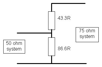Fig. 5. Pad for matching 50 and 75 ohm systems. Suggestions for practical values: 43.3R is made up from series 33R and 10R; 86.6R is made up from series 69R and 18R. In either direction, the insertion loss is 4.6 dB.   Fig. 6a The simplest possible set-up for S-meter calibration. Each unit must match the same impedance and the connections are made using co-axial cable of the same impedance. Thr 6dB attenuators are to isolate any impedance mismatch at the receiver or generator from the variable attenuator. Earth connections are made with heavy copper braid.   Fig. 6b. A more complicated set-up with the generator and receiver being matched to 75ohms, while the available attenuators are 50ohms. Two pads as shown in Fig. 5 have been used.