Please feel free to print out and keep this page.....

Why calibrate?

Measurements have units; the recognised unit of relative signal strength is the decibel (dB). In order to compare the measurements from different observers they must be given in dB. In addition the calibration of your equipment is a good exercise in the art of experimental science, and can be useful for giving objective reports of QSB, antenna comparisons, processor compression etc. The guy at the other end will be impressed!

What is an S-point?

First question, has your receiver got a good S-meter? It is possible to convert a report of three apples, two oranges and a cherry into dB, but I suggest that a LED display containing perhaps 8 levels is not going to be very accurate. Most S-meters are marked in "S-points" (1 to 9) and then numbers of dB above S9. In my experience, very few are meaningful in having a consistent value of the S-point. One exception is my Kenwood-Trio TS-820-S, which follows very linearly a calibration of 1 S-point = 6 dB, the original definition. You could however just ignore S-points and calibrate directly in dB.

The Signal Source

You will need a stable signal source within the range of the receiver. This could be a signal generator, a crystal calibrator, or another transmitter run at very low power, An off-air signal is the last thing to consider, because propagation is never stable, certainly not to a few dBs. A simple two-transistor HF source is given in [2], p. 8-2. The source must be well screened; if you are to successfully calibrate down to the bottom end of the range there must be no leakage of signal around the attenuator.

Adjusting Signal Level - Signal Generator

If you are using a commercial signal generator, this may have its output already calibrated in dB relative to some fixed level e.g. 1 mW. It may be calibrated in power level, normally microwatts (mW), in which case these must be converted to dBs by the formula 10 log₁₀(P2/P1), where P1 is an arbitrary power level. Sometimes the output of a generator is marked in volts, milli-volts (mV) or micro-volts (mV), These may be converted to a dB power ratio, remembering that power is proportional to V², so dB=20 log₁₀ (V2/V1). Again, V1 may be chosen arbitrarily. For those not mathematically inclined, many electronic reference books give tables of linear ratios of power and voltage corresponding to a range of dB values, e.g. [4] p.11-6. Any outside this range can be easily derived by adding dB and multiplying the corresponding ratios. Thus, 23 dB = 10dB + 10dB + 3dB = 10 x 10 x 2 = x 200 (power), or x 14.2 (voltage).

Adjusting Signal Level - Uncalibrated Output

If your signal source does not include a calibrated output, you will need a variable attenuator. Generally these are switched, and should have a minimum step of 1 or 2 dB. You will need in addition fixed attenuators to add up to about 100 dB.

It is important to note that attenuators only give the correct value when the input and output are correctly terminated by the impedance for which they are designed. You cannot rely on the impedance at the antenna socket to be its nominal value; the same is true of many signal sources. We overcome this by using fixed attenuators either side of the variable attenuator; this "isolates" it from any incorrect impedance. The larger the attenuators, the better the isolation. However, the signal source has to be beefy enough to be able to supply full scale deflection on the S-meter with these attenuators in line. At least 6dB attenuators are recommended, though 3 dB attenuators can be used if signal strength is a problem.

Matching Impedances

Most of the amateur radio equipment today matches a nominal 50 ohm impedance, though older equipment (and many signal generators) will be 75 ohm impedance. You may well find surplus 75 ohm attenuators much cheaper than their 50 ohm counterpart.

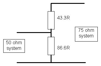
You can use either 50 or 75 ohm attenuators (but not in combination) ⁵. Where the nominal impedance of either the receiver or the generator differ from the impedance of the attenuators, you need a matching unit. Fig. 1 shows a circuit designed to match 50 ohms to 75 ohms and vice versa, It consists of merely two resistors, which should be mounted using the connectors as supports in a small metal box (a soldered-up tin is ideal), the leads being kept as short as possible. Take care not to overheat the resistors when soldering them in position.

Fig. 1. Pad for matching 50 and 75 ohm systems. Suggestions for practical values: 43.3R is made up from series 33R and 10R; 86.6R is made up from series 69R and 18R. In either direction, the insertion loss is 4.6 dB.

Connections

Connect your signal source to the input of your variable attenuator via a fixed attenuator, and the output of the attenuator again via a fixed attenuator to the receiver, using good quality coaxial cable of the correct impedance. If you are using a calibrated generator, the variable attenuator and one fixed attenuator are omitted. It is best if you place the receiver and source some distance apart, to minimise direct pick-up. Make sure also that any units supplied with an earth connection (usually the signal generator and receiver, but also possibly the variable attenuator) are electrically joined together, preferably with thick braid, and then to a good earth connection.

The simplest set-up using an uncalibrated signal source is shown in Fig. 2a. An example using a signal source and receiver designed to match 75 ohms, but retaining the 50 ohm attenuators, is shown in Fig 2b.
 
 

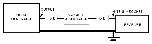
Fig. 2a The simplest possible set-up for S-meter calibration. Each unit must match the same impedance and the connections are made using co-axial cable of the same impedance. Thr 6dB attenuators are to isolate any impedance mismatch at the receiver or generator from the variable attenuator. Earth connections are made with heavy copper braid.
 

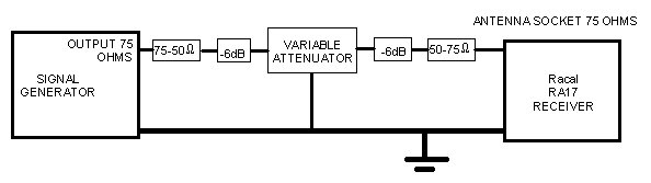
Fig. 2b. A more complicated set-up with the generator and receiver being matched to 75ohms, while the available attenuators are 50ohms. Two pads as shown in Fig. 1 have been used.
 

Setting up and Checks

Leave your signal source and receiver switched on for at least half an hour before calibration, to let them reach a stable temperature. During this time you can do the following.

Tune your receiver to the frequency of the signal source, choosing a quiet frequency if the source is tuneable. With the variable attenuator set to zero, turn up the output of the signal generator to ensure you reach full scale deflection of the S-meter. If not, you need a stronger signal source. Now unplug the output of the variable attenuator moving the cable well away. Check that there is no deflection of the S-meter when you tune the receiver through the generator frequency. If there is, you have leakage of the RF past the attenuator circuit. You must eliminate this before proceeding, by improving your screening or increasing the distance between generator and receiver. If all else fails, it may be necessary to wind each end of the coax on ferrite toroids to eliminate currents on the outer conductor of the coax.

Preliminary Adjustments

Most S-meters have provision for adjusting the zero reading and the sensitivity. Look in the handbook, if you have one, otherwise look for two adjustable potentiometers in the meter circuit. If you have any doubt about the function of any adjustable, DO NOT MOVE IT. Instead, calibrate the S-meter as it is, skipping the next two paragraphs.

Zero Adjustment

With the receiver connected to an attenuator (so that the antenna socket is correctly terminated), but with the signal source off, you should hear only receiver noise. Adjust the zero setting so the S-meter reads S1. The reason I prefer my S-meter reading 'S1' on noise is that one can often read signals which do not move the S-meter, and yet one cannot give a report of R3 or R4 and S0!

Sensitivity Adjustment

First work out the dynamic range of the scale; there are eight S-points between S1 and S9, spanning a range of 8 x 6dB = 48dB. Add on the "dB's over S9", e.g. my S-meter reads up to S9 + 40dB, making a total of 88 dB. Subtract 6dB (one S-point) from the value calculated. You now need to adjust the S-meter sensitivity such that a change of attenuation equal to this value produces a change from S2 to full scale. If the adjustment does not cover this, set it as close as you can. You will need to vary the level of the source to achieve this, or use a combination of attenuators if the output is not adjustable.

The Calibration

Next adjust the output of your signal generator or attenuation to produce full scale deflection of the S-meter (e.g. S9+40dB in my case). Now increase the attenuation (or reduce the calibrated output) until the next division is reached (S9+20 dB in my case). Make a note of this value. Repeat for each subsequent meter division. If you are using a variable attenuator, you will eventually run out of range. You must either add fixed attenuators, or if these are not available, re-set the output of your generator, To do this, note the position of the S-meter, reset the variable attenuator to zero, and reduce the generator output to get to the same point on the scale. You must now add to subsequent values, the number of dBs you removed.

Plot the Results

You are now able to plot a graph of S-meter reading along one axis against added dBs. You should be able to draw a smooth line through the points. If a straight line suffices, then the meter is linear in dB; if it is curved, you may want to use a flexi-curve or French curve to obtain a smooth fit. If you have a computer with a curve fitting program, then try a polynomial with increasing powers until the fit is satisfactory.

Now measure the difference in dB between each point and the line (positive one side, negative the other); if it is a good fit, these differences should add up to near zero. If one of these values is very large, that is the point is a long way from the smooth line, then go back and check this point and if necessary the values of the attenuators.

The so-called "standard" or RMS (Root-Mean-Square) deviation of the points from the curve is a measure of its accuracy. If you used a computer fit, the program should give you this value. If not, square the differences you have just calculated (they are now all positive), add them, divide the sum by the number of points less one, and take the square root of this number. If your calibration was properly done, this number should be between 1 to 3 dB.
 

Some useful References

[1] D. Emerson, G3SYS/ AA7FV, "Radio Observations of Two Solar Eclipses", QST (Feb 1995) pp. 21-26.

[2] "World Radio TV Handbook 1998", ISBN 0-823-079-97-7 (52nd edn; Billboard 1998).

[3] H.L. Gibson, "Test Equipment for the Radio Amateur" (2nd edn; RSGB 1978).

[4] G. H. Grayer, Chapter 2 "VHF/UHF Propagation" of "The VHF/UHF DX Book", ISBN 0-952-046-80-6 (Ed. I.F. White G3SEK), p. 2-62.

[5] J. Morris, G4ANB, "Locator System for VHF and UHF"; Radio Communications 56, 11 (November 1980) pp. 1160 - 1163.

[6] J.C.D. Marsh, "Measurement and analysis of radio emission from the quiet sun"; J.B.A.A. 108, 6 (December 1998) pp. 317 - 319.